Use the safety stock calculator ↓
The safety stock formula for variable daily demand and a fixed replenishment lead time is SS = z × σd × √L. Here, z represents the target cycle service level, σd is the standard deviation of daily demand, and L is lead time in days. It is useful only when those assumptions fit your data.
If lead time also varies, the calculation changes. If you only have maximum and average values, you can use a simpler estimate, but that number does not establish a particular service level.
Choose the formula after checking how you place orders and when replenishment becomes usable. Using factory completion as the end of lead time, for example, leaves transit and receiving demand out of the calculation.
How much buffer does your stock need?
Estimate safety stock and a reorder point using the method that fits your data.
The extra buffer for uncertainty
Behind the numbers
Safety stock and the final reorder point are rounded upward to whole units. Calculations use unrounded values.
Seasonal, intermittent or correlated demand and delays need a different analysis. Test the result against actual replenishment cycles.
Which safety stock formula should you use?
Safety stock is the buffer held above expected demand during replenishment. It covers uncertainty; it is not the full amount you expect to sell while waiting for an order.
| Situation | Starting method | Main limitation |
|---|---|---|
| Only maximum and average history available | Maximum-average estimate | No calibrated service probability |
| Variable demand, fixed lead time | z × σd × √L | Needs a suitable demand model |
| Variable demand and lead time | z × √(L̄ × σd² + d̄² × σL²) | Assumes independent demand and lead time |
| Seasonal, intermittent, or correlated demand and delays | Model lead-time demand or forecast errors directly | Needs a different analysis, not a plug-in correction |
The first two calculations are described in SPS Commerce’s safety stock guide. The variable-lead-time expression uses the independent-variability approach explained by Peter L. King in APICS magazine. APICS safety stock article, hosted by MIT.
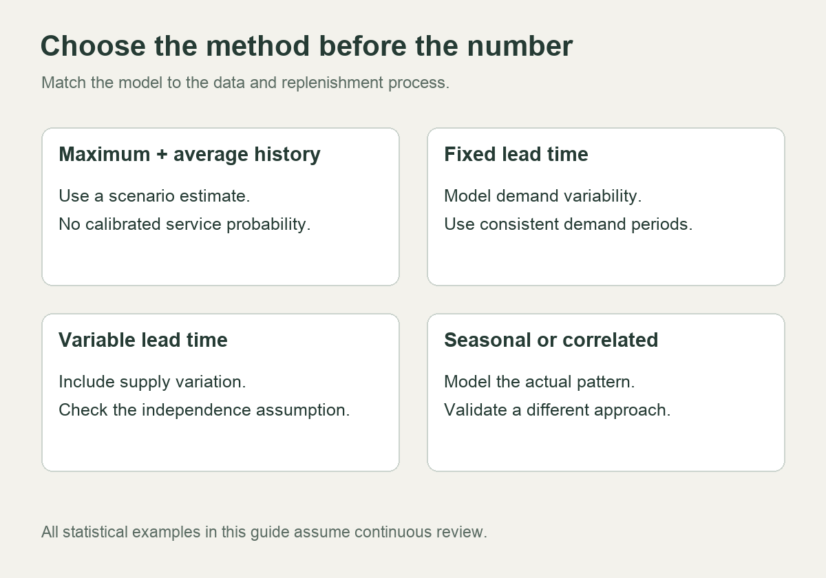
The statistical examples below assume continuous inventory review, reasonably stable demand, independent daily demand increments, and an approximately normal distribution of demand over the protection period. They are starting models to validate against your operation, not promises that a chosen buffer will deliver a stated result.
Prepare the inputs before calculating
Use one SKU, one replenishment destination, and one consistent unit of measure. Combining unrelated sizes or locations can hide the shortage you are trying to prevent.
| Symbol | Meaning | Unit in this guide |
|---|---|---|
| d̄ | Average demand per day | Units per day |
| σd | Standard deviation of daily demand quantities | Units for a one-day period |
| L or L̄ | Fixed or average replenishment lead time | Days |
| σL | Standard deviation of replenishment lead time | Days |
| z | One-sided normal quantile for cycle service level | No unit |
| SS | Safety stock | Units |
Measure lead time to usable stock at the location being replenished. A supplier’s production estimate alone may omit order processing, transport, receiving, or inspection. If your measurement ends at warehouse arrival but items remain on hold for two days, the replenishment process is not finished when your spreadsheet says it is. Keep calendar conventions consistent. Daily demand measured across all calendar days needs a compatible lead-time measure. Do not combine weekly demand variability with lead time in days without converting the periods correctly. Also check what your sales history records. Zero sales during a stockout do not prove that demand was zero. Returns, bulk orders, and promotions can distort the series if you treat every transaction as ordinary daily demand.
Method 1: the maximum-average estimate
The simple version is: SS = (maximum daily demand × maximum lead time) − (average daily demand × average lead time) For an illustrative SKU, suppose maximum daily demand is 45 units, maximum lead time is 12 days, average daily demand is 30 units, and average lead time is nine days: SS = (45 × 12) − (30 × 9) = 270 units. This estimate effectively builds a buffer around sustained peak demand across the longest observed lead time. It can be large. A single unusual promotion or delayed shipment can substantially change the result. Use it as a transparent scenario estimate when those inputs are all you have. Record the observation window and why the extremes are relevant. Do not label the resulting 270 units a “95% service level” calculation: there is no probability target in this formula. Nor does the largest value in your historical sample establish the worst possible future event. A short, quiet history can make this estimate too small.
Method 2: variable demand with a fixed lead time
For independent daily demand and constant lead time: SS = z × σd × √L The square root matters. Under the independence assumption, daily demand variances add across days; the standard deviation therefore grows with the square root of the number of days. Use these hypothetical inputs:
| Input | Value |
|---|---|
| Average daily demand | 30 units |
| Daily demand standard deviation | 8 units |
| Fixed lead time | 9 days |
| Target cycle service level | 95% |
| z, rounded | 1.645 |
The calculation is: SS = 1.645 × 8 × √9 = 39.48 units. Round upward to 40 units for an indivisible product. Expected demand during the nine-day lead time is 30 × 9 = 270 units. The corresponding reorder point is 270 + 40 = 310 units, before any separate implementation adjustments.
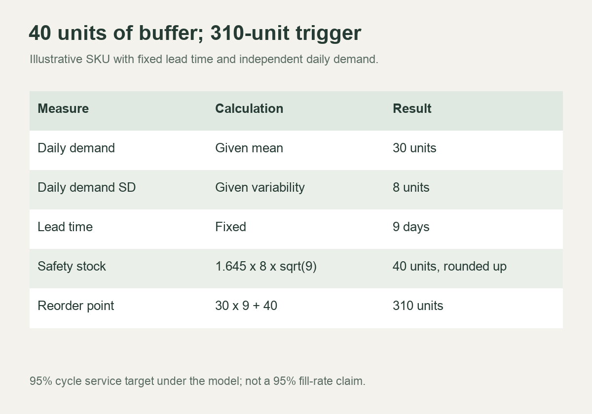
These values have different jobs. The buffer is 40 units. The expected lead-time demand is 270 units. The reorder trigger is 310 units. None of those figures, by itself, tells you how many units to buy on each order.
A spreadsheet version
If B2 contains average daily demand, B3 daily demand standard deviation, B4 fixed lead time, and B5 the cycle service target entered as 95%, the safety-stock calculation in common English-language spreadsheet syntax is: =ROUNDUP(NORM.S.INV(B5)*B3*SQRT(B4),0) The reorder point is: =B2*B4+B6 Here, B6 contains the rounded safety-stock result. Validate the inputs before using the sheet: quantities and lead time must use compatible periods, and the service target must be between 0 and 1. This simple buffer model is intended for targets above 50%, not for producing negative safety stock. The spreadsheet uses a more precise normal quantile than the displayed 1.645. Both versions round to 40 units in this example.
Method 3: demand and lead time both vary
If demand and replenishment lead time are independent, a common normal-approximation calculation is: SS = z × √(L̄ × σd² + d̄² × σL²) The first term captures demand variation across the average lead time; the second captures exposure to lead-time variation. Keep the same daily-demand inputs and nine-day average lead time, then vary only the lead-time standard deviation.
| Lead-time standard deviation | Calculation using z = 1.645 | Rounded buffer |
|---|---|---|
| 0 days | 1.645 × √(9 × 8²) | 40 units |
| 1 day | 1.645 × √(9 × 8² + 30² × 1²) | 64 units |
| 3 days | 1.645 × √(9 × 8² + 30² × 3²) | 154 units |
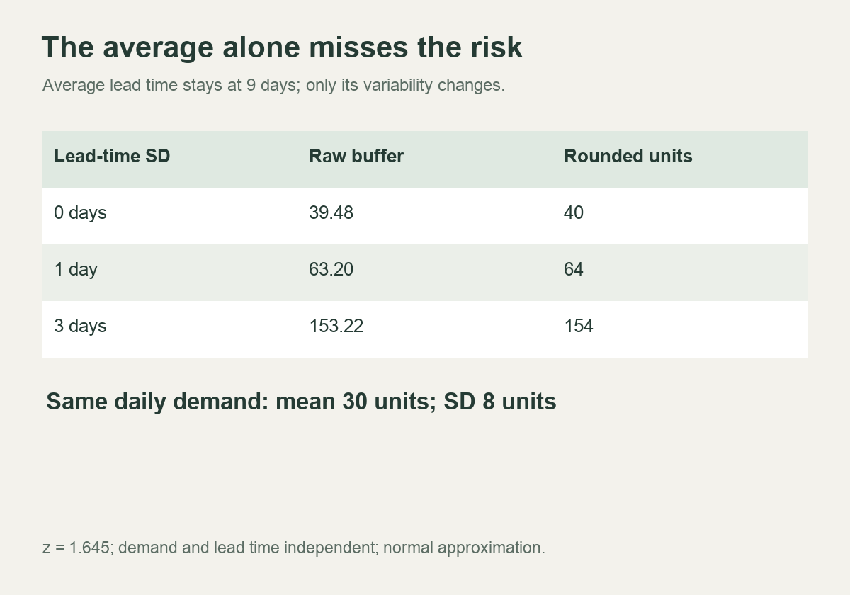
The average lead time is unchanged in all three rows. Its variability changes the buffer. Using only “nine days on average” would miss that difference. This example is a sensitivity calculation, not evidence that reducing lead-time variability will always produce the same savings. The result depends on the SKU’s demand pattern and other inputs. If demand surges also cause supplier delays, the independence assumption is doubtful. Do not force that situation into the formula or add an arbitrary percentage afterward. Consider modeling the observed joint behavior, or simulating replenishment with realistic demand and delay scenarios. Sparse data may require a deliberately conservative operating decision while you collect better evidence.
What does a 95% service level mean here?
These z-based calculations target cycle service level: the probability of avoiding a stockout during a replenishment cycle under the model. A 95% target does not mean that exactly 95% of units, orders, or customers will be fulfilled immediately. Fill rate measures how much demand is satisfied from stock. Stockout frequency and stockout size are different questions. Chris Caplice’s MIT logistics lecture defines cycle service level as the probability of no stockout in a replenishment cycle and item fill rate as the fraction of demand filled from on-hand inventory. MIT lecture on probabilistic inventory. For reference, one-sided normal quantiles are approximately 1.282 for 90%, 1.645 for 95%, and 2.326 for 99%. Choose the target based on the consequences of shortage and the cost of holding stock. There is no single correct target for every product.
Turn the buffer into a replenishment rule
The usual continuous-review relationship is reorder point = expected demand during lead time + safety stock. Shopify’s min-max inventory guide also separates the reorder threshold from order quantity. In a basic continuous-review model, compare the threshold with inventory position, commonly defined as on-hand stock plus on-order stock minus backorders. Confirm how your system treats allocations, unavailable stock, and incoming orders. If its “available” figure already deducts a commitment, subtracting that commitment again would distort the trigger. For example, with 220 usable units on hand, 100 on order, and 20 backordered, inventory position is 300 units. That is below the illustrative reorder point of 310, even though the number physically on the shelf is a different figure. This simple example assumes the incoming supply is valid and appropriately timed; a late or uncertain PO needs separate attention. If you review inventory only once a week, demand can continue between reviews before a new order is placed. The protection period then generally includes the review interval as well as replenishment lead time. Use a periodic-review policy designed for that process rather than copying the continuous-review threshold unchanged.
Check the policy against purchasing and receiving reality
Before adopting the result, write down the SKU, destination, data window, formula, service metric, rounding rule, and review owner. Recheck it when demand changes materially, the supplier changes, or the replenishment route changes. Replay past replenishment cycles where data permits. Examine when shortages would have occurred, how large they would have been, and what stock the rule would have required. Treat that as a historical check; it cannot establish future performance if the operating conditions have changed. Supplier minimums belong in the order-size decision. If an MOQ forces a much larger purchase than the demand plan supports, explore smaller replenishment orders with Chinese suppliers alongside price, packaging, and freight tradeoffs. Extra cycle stock created by a large order is not automatically a carefully designed safety buffer. Receiving delays also deserve attention. When discussing China warehousing and fulfillment, agree which milestones will be recorded: arrival, count completion, inspection release, and availability for dispatch. Those timestamps can improve your lead-time input. Confirm the reporting arrangement for your account rather than assuming a warehouse service includes forecasting.
Frequently asked questions
Is safety stock the same as minimum stock?
Not always. Software and businesses use “minimum” differently. In this guide, safety stock is the uncertainty buffer; the reorder point includes expected lead-time demand as well. Check the definition before copying a number into a system field.
Can I use a fixed percentage of sales?
You can set a provisional operating buffer that way, but a percentage alone does not account for demand variability, replenishment variability, or a defined cycle service target. Record it as a management assumption and review its results.
What if demand is seasonal or intermittent?
Do not treat an annual average and standard deviation as a complete model. For seasonal items, examine forecast errors over the relevant replenishment horizon. For intermittent demand, use a method that represents the many zero-demand periods and occasional orders. Validate the resulting policy against the service measure you actually need.